A Python library that builds 3D-printable parts from equations instead of meshes, and a case study that takes one design from optimiser to end-to-end CFD.
The library
Python · GPU · since 2024
A Python library for designing 3D-printable lattice parts, which most CAD tools handle poorly. Shapes are defined by equations instead of triangle meshes, and rendered live on the GPU.
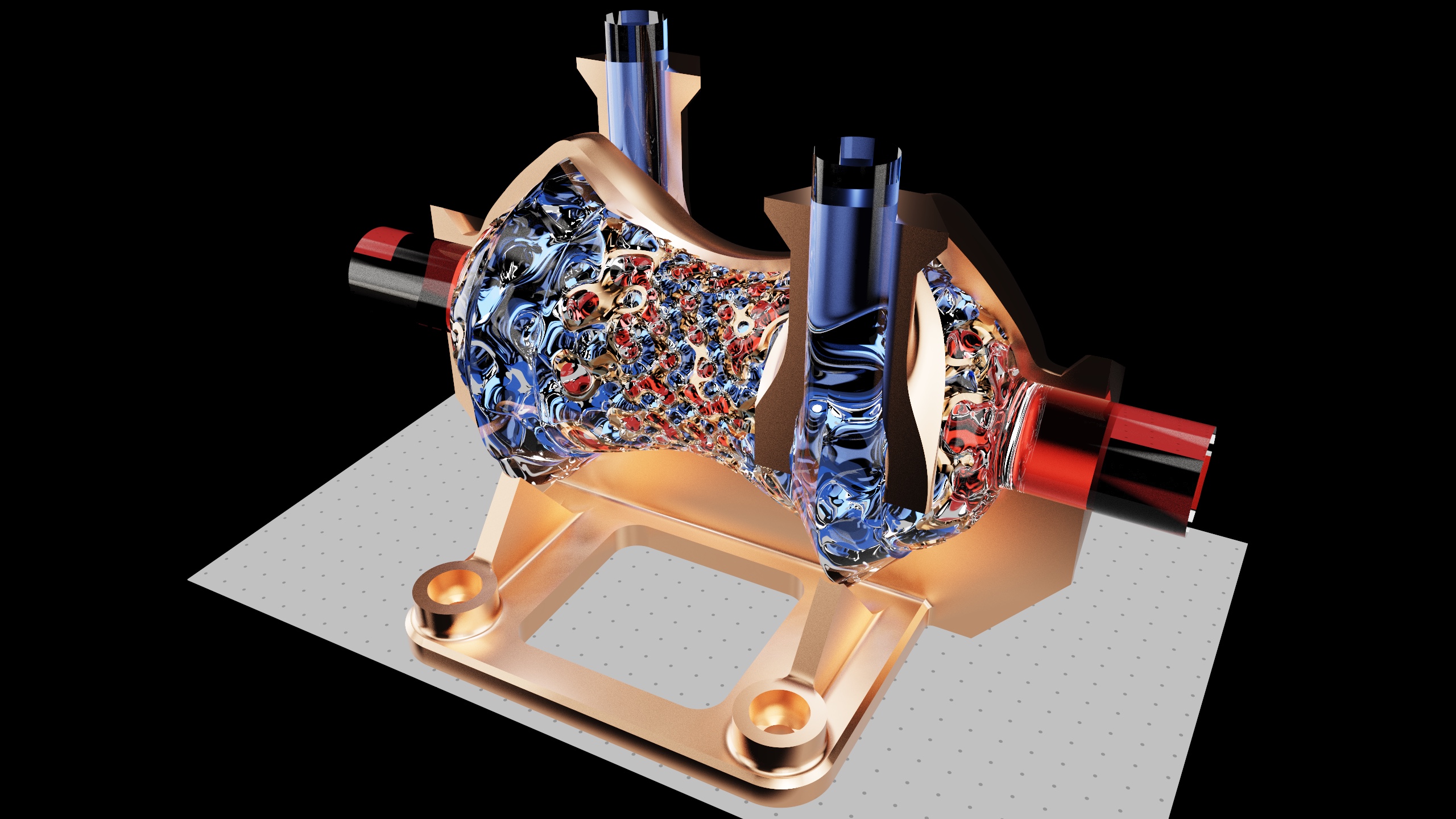
Graded-gyroid counterflow heat exchanger, path traced in FluidForm: tinted glass fluids either side of a copper-coated gyroid wall. The portfolio has it live in your browser.
Every shape, from a box to a gyroid lattice to an imported STL, is a signed distance field evaluated in real time with Taichi (WIP Rust port). Parts combine through boolean CSG and TPMS infills, update instantly in a physically based ray marcher, and export to STL for printing. I wrote it to design printable lattice parts for additive manufacturing without fighting mesh topology, but geometry defined in code allows much more: a part can be driven by parameters, sized by an optimiser and handed straight to a simulation, as the micromixer below and ColdFlow show.
Geometry
25+ SDF primitives, smooth CSG, domain warps
Lattices
Gyroid, Schwarz P/D, Lidinoid, Neovius, Fischer–Koch, Split-P or whatever you can define
Render
BVH ray marcher, progressive path tracer
Quality
777 tests · 544 commits
Source
GitHub ↗ coming soon
Case study · optimisation
An organic two-tree micromixer, sized for two fluids of different viscosity and volume
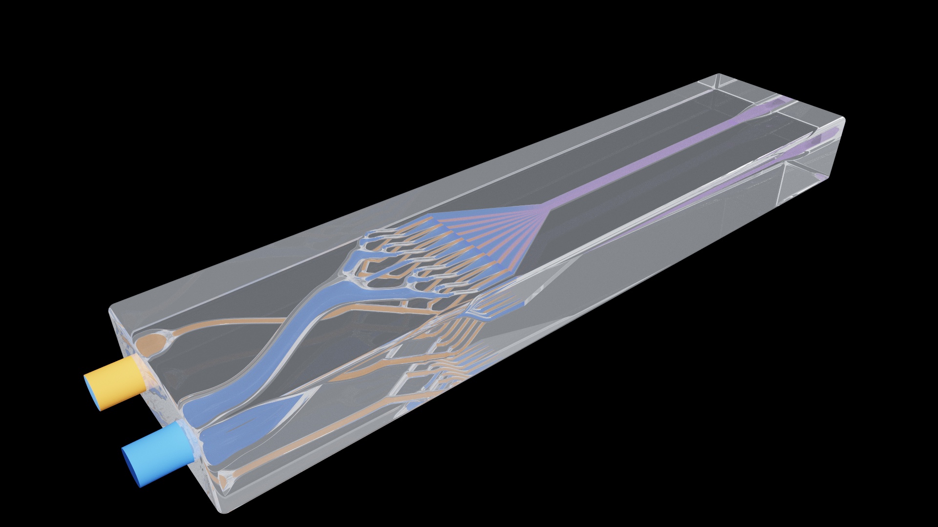
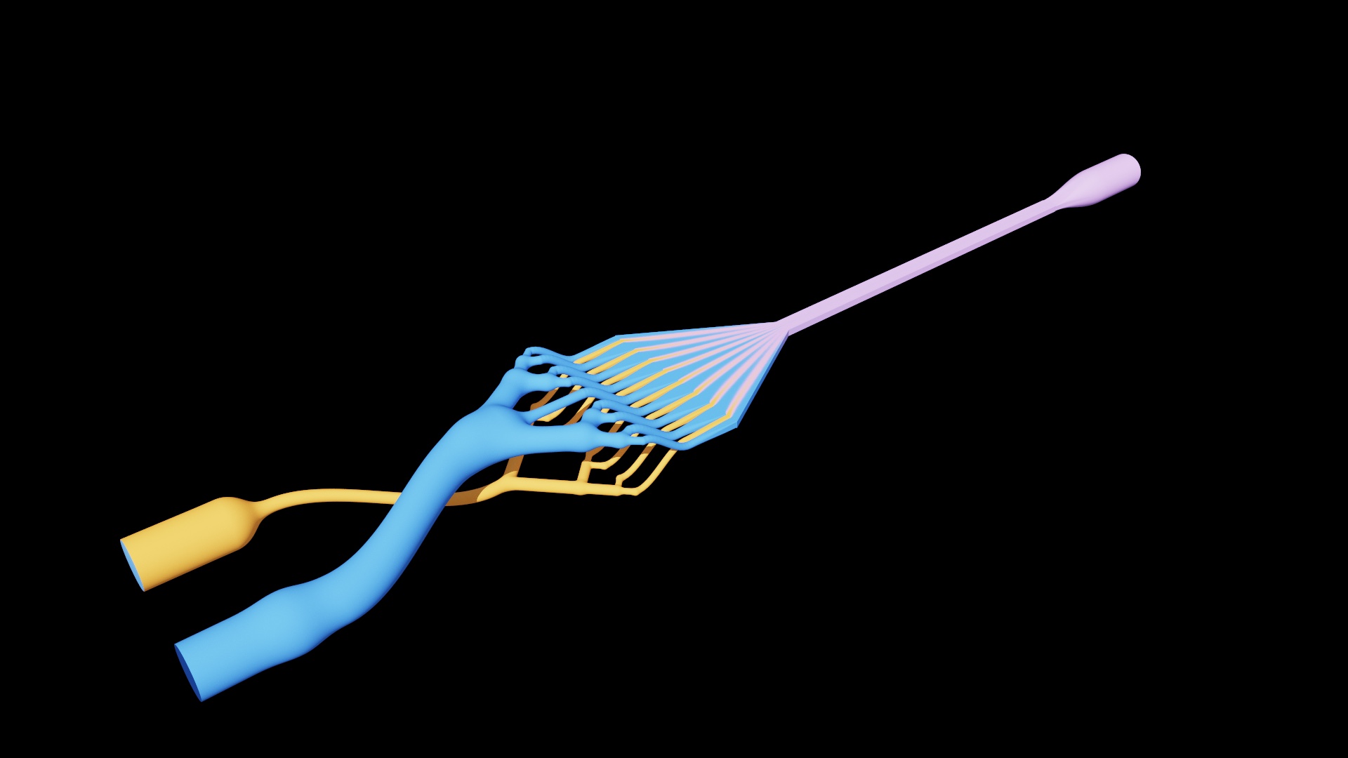
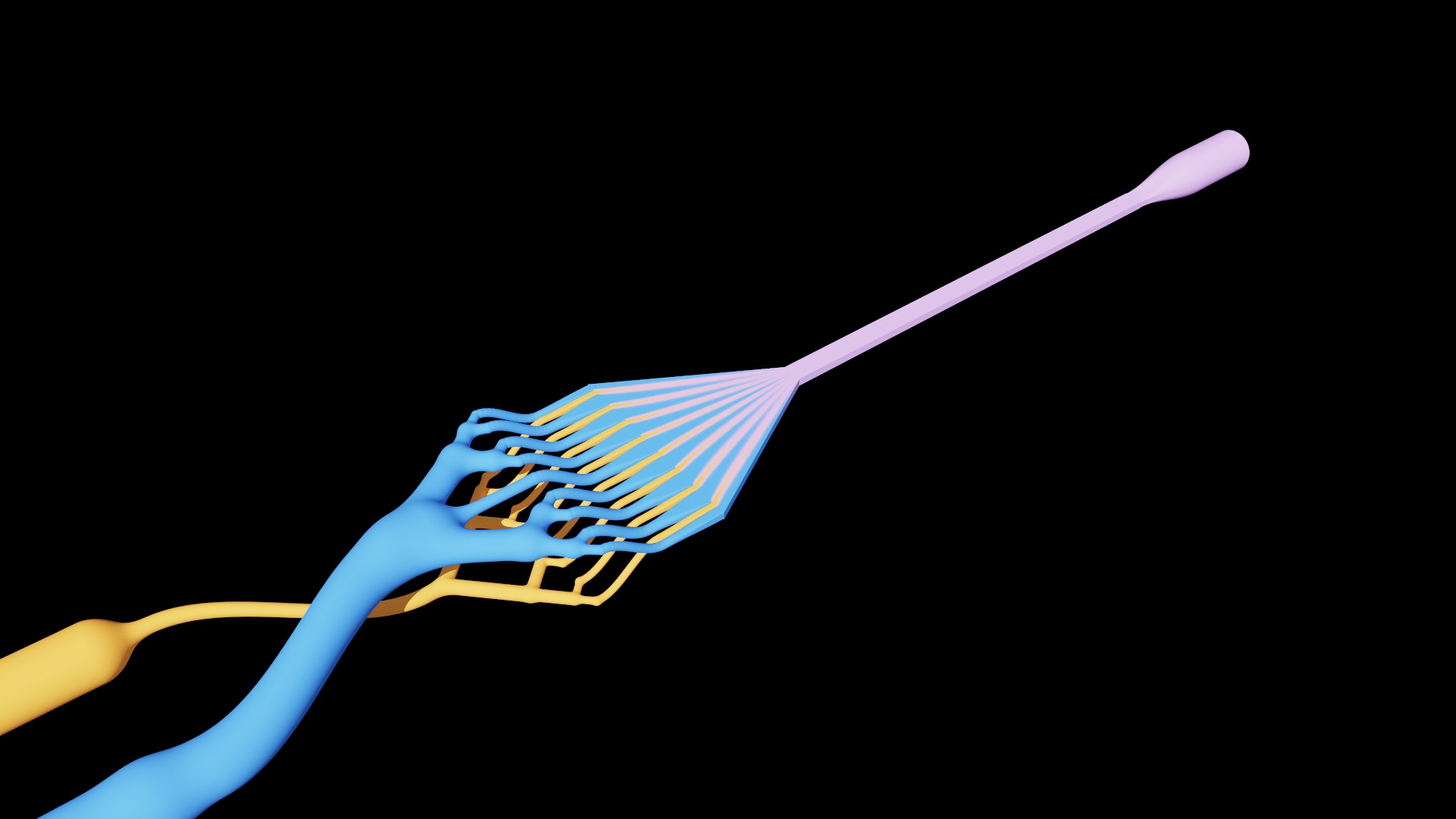
Two fluids are wanted in the ratio 1 part A to 3 parts B and mixed in a few millimetres. Each is split by its own branching tree of round tubes, three smooth forks into eight leaves for A and a nine-leaf tree for B. Both inlets are on the left, side by side, and each trunk then eases onto its own layer, A below and B above. Near the end every leaf flattens from a round tube into a rectangular slot, and the slots meet the flat channel edge to edge as alternating stripes, each fluid's slot as wide as its share of the flow (a quarter for A, three quarters for B, with half a B slot against each wall), and the channel narrows after the stripes form, which thins them and mixes the two. Both inlets sit at one pressure, so the volume each fluid delivers depends only on its tree's resistance, and resistance scales with viscosity. A is water-like (1.2 mPa·s) and B is a thicker reagent (4.0 mPa·s). An optimiser sized every tube to deliver exactly the wanted ratio, and the result is modelled and rendered in FluidForm.
1 : 3wanted volume ratio of A to B, delivered exactly at one shared pressure
3.3×viscosity of B over A, which makes B's tree much wider than A's
8mmof mixing section at 30 µL/min: 99% mixed in CFD (a plain channel needs 63 mm)
0.66kPapressure needed, the quantity the optimiser minimises
Resin bodyFluid channels
The mixer as it would print in clear resin, and the fluid it carries. Drag to remove the resin. Fluid B (blue) takes the wide upper tree and fluid A (orange) the fine lower one; their leaves flatten into slots that meet the mixing channel edge to edge. The channel is coloured by the simulated mixture, from the stripes at the slots to violet where the two are fully mixed. Every dimension is to scale except the gap between the layers, which is stretched.
Tube diametersstems, levels, leaves
Hydraulic networkflow of A and B, pressure
Mixingtime to 99%, from the stripe widths
Constraintsratio, length, volume, taper
Objectiveleast driving pressure
SLSQP on log-diameters; each level held between 0.6 and 1 times its parent, so it stays a tree
01 · Viscosity
The same trees would deliver the wrong volumes
At a shared pressure the flows split as the inverse of the resistances, and a thicker fluid has more resistance in the same tube. Trees built for two water-like fluids at equal volumes would deliver 3.3 parts of A to 1 of B with these fluids, ten times too much A against the 1 to 3 wanted.
02 · Not Murray's law
The tubes are sized for the fluids, not for one fluid
Murray's law gives the tree that moves a single fluid with the least pressure. Here the two trees must differ: B's stem is 538 µm across and A's is 157 µm, and they taper to leaves of 116 µm and 74 µm. The optimiser keeps each level between 0.6 and 1 times its parent, so both still read as trees.
03 · Mixing
Narrowing the stripes does the work
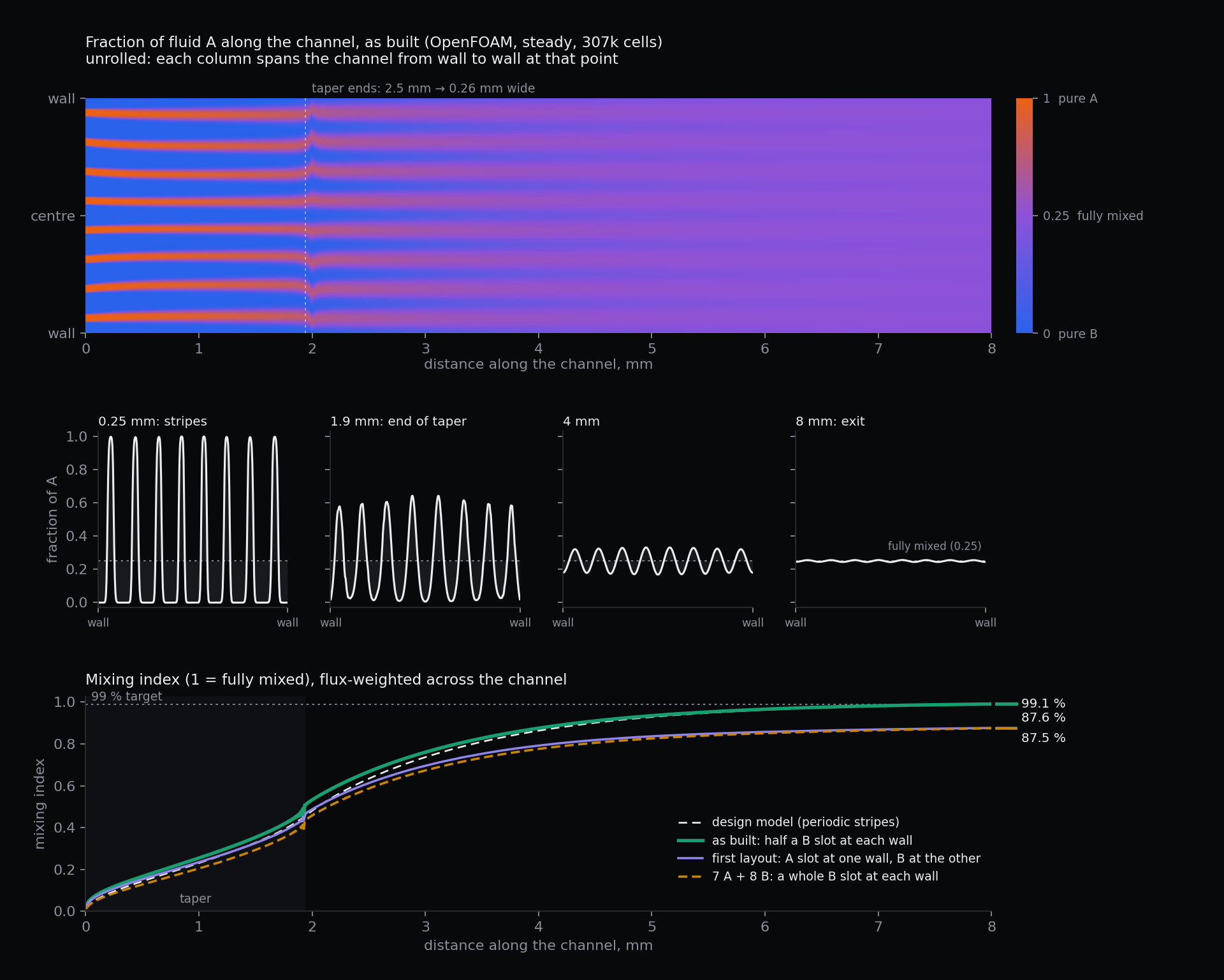
Eight stripes of A sit between B's, 312 µm per pair, with half a B stripe against each wall. Diffusion across a stripe sets the mixing time, so after the stripes form the channel narrows from 2.5 mm to 0.26 mm, which thins every stripe by the same factor. The design model puts that at 99% mixed in 8 mm, where a plain channel would need 63 mm; the CFD below confirms it, after catching a flaw in the first layout.
04 · Result
Exactly 1 to 3, at less than a kilopascal
The design delivers 1 : 3.00 at 0.66 kPa and 30 µL/min, and holds 1.6 µL of fluid in its tubes and channel. In the earlier flat-channel version of this study, two forks per tree needed about nine times the pressure and four did not fit in 2.5 mm, so three is the sweet spot.
Results · delivered volumes at the same pressure
Design
A : B delivered
Against wanted
Equal volumes, water-like fluids
3.33 : 1
A 10× over
Right volumes, viscosity ignored
1.11 : 1
A 3.3× over
Optimised
1 : 3.00
exact
Ignoring either the viscosity or the volumes delivers the wrong ratio; sizing for both delivers the wanted one. The narrow A leaves are the sensitive part when the print varies.
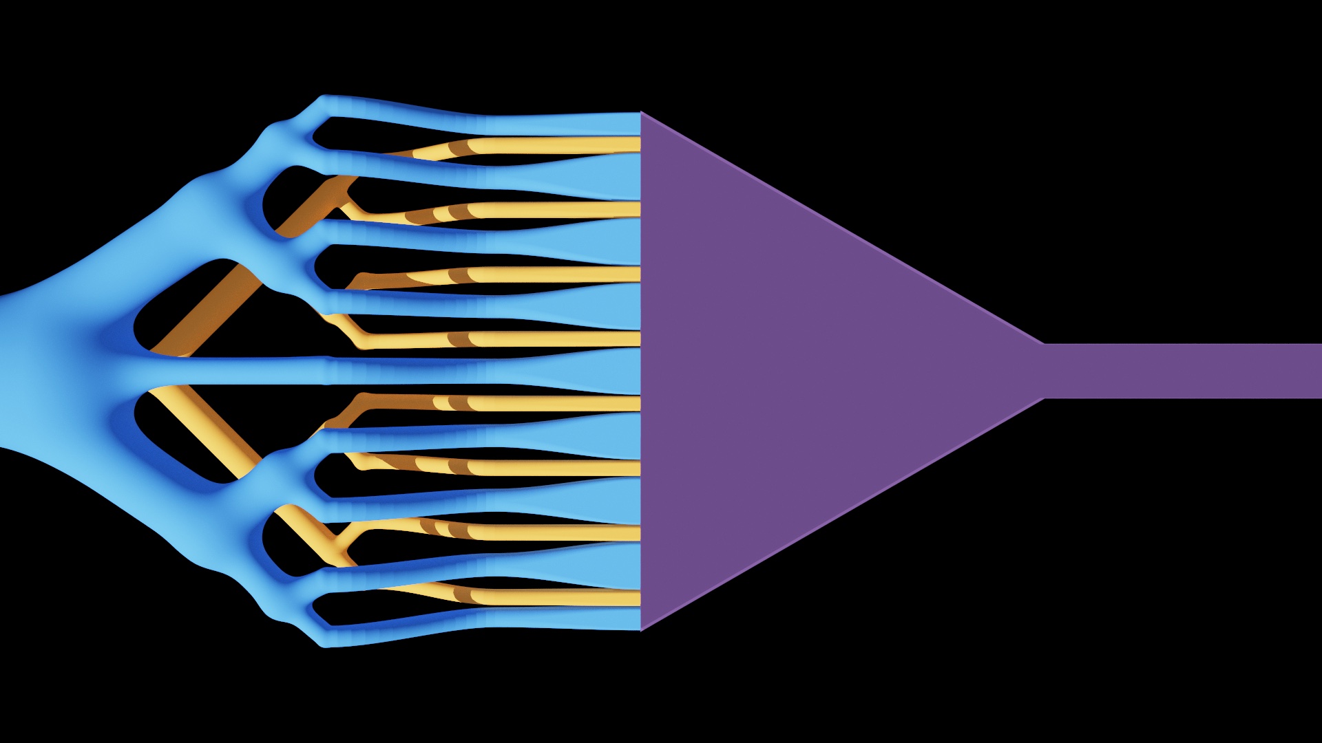
The branches and the collector from above. Each leaf flattens from a round tube into a slot along the collector's edge, and the collector narrows from 2.5 mm to 0.26 mm over 1.9 mm.OpenFOAM simulation of the mixing, steady state, 307k cells. Top: the fraction of A along the channel, unrolled so each column spans it wall to wall, from pure B (blue) through fully mixed (violet) to pure A (orange). Middle: across the channel at four stations. Bottom: the mixing index for the layout as built, the first layout and an alternative, against the design model. Tap the figure to open it full size.
The mixing is simulated in OpenFOAM on the channel in two dimensions. In a 0.1 mm deep channel the depth-averaged flow is a potential flow in the plane, so potentialFoam gives the velocity and scalarTransportFoam carries the fraction of A with the mixed stream's diffusivity, using the real slot pattern at the inlet. A 77k-cell and a 307k-cell mesh agree on the mixing index at the exit to 0.02%. The channel is 99.1% mixed at 8 mm, matching the design model. The first layout did not: it ended on a full A slot at one wall and a full B slot at the other, and the simulation found it only 88% mixed, a slow imbalance across the whole width. The model assumes a periodic stripe pattern, which needs the walls to sit mid-way through a slot. A full B slot at each wall (7 A and 8 B) did not help (87.5%), so B's tree became a nine-leaf tree with half-width slots against the walls, its end two leaves carrying half flow and sized so the 1 : 3 ratio holds.
The flows are checked against an independent calculation: a solve of every tube and channel segment in both trees agrees with the closed-form flows to round-off. With random print error on every tube, a common bias up to ±3 µm and 2 µm per tube, over 1,000 chips, the delivered ratio has a standard deviation of 3.6%, and the flow among a tree's eight leaves varies by 8% for A and 5% for B. The hydraulic model uses straight round tubes and leaves out the curved drop of each leaf, the round-to-slot transitions, the flow at the junction and the outlet; the mixing CFD above is two-dimensional and depth-averaged. Nothing has been printed or tested. Earlier versions, with flat channels, a single focusing stage and herringbone grooves, are kept on a branch of the repository.
The trees themselves are simulated in 3D as well. Each tree's fluid volume is taken from the model's own surface, meshed with snappyHexMesh (350k and 790k cells) and solved with simpleFoam at the same pressure drop. Every leaf carries its intended share, but the totals did not match the design model: the leaves open into slots wider than their tubes, which the straight-tube model ignores, so B flowed 27% faster than designed and the pair delivered 1 : 3.69 instead of 1 : 3. Scaling B's tube radii and re-running the simulation closed it in steps (1 : 3.69, then 1 : 2.70, then 1 : 3.003 at 0.946 of the radii). Softening every fork's fillet then changed the resistance again, to 1 : 3.085, so B was recalibrated once more, to 0.940 of the design radii. The final trees deliver 1 : 3.0007 (A 47.7 µL/min, B 143.2 µL/min at 500 Pa), A's leaves within 0.5% of equal and B's whole leaves within 1.2%. Calibrating after the last geometry change, not before, is the lesson.
End-to-end 3D simulation of the whole device on one mesh, coloured by the mixture: orange is pure A, blue pure B, violet fully mixed.
Finally the whole device is simulated end to end on one 1.86M-cell mesh: both trees, the slots, the channel and the outlet, with the flows set to the calibrated values and the mixture carried to steady state. It reaches 98.3% mixed at the exit, a little under the 2D result, most likely from the real end leaves running slightly short. At this mesh size the stripes are thinner than a cell by the end of the taper, so the 3D run overstates the mixing there; the resolved 2D run above remains the measure of how fast it mixes.